Apologies, this page only works in landscape mode.

Intro image here

Figure 1: Longitudinal Magnetization Graph of longitdunal magnetization versus time for tissues with short (black), medium (blue), and long (red) T1 times. The longitudinal magnetization grows from zero to its maximum value over time. Tissues with a longer T1 time take longer grow to their maximum value. This growth, also called recovery, begins to occur whenever there is sub-maximal longitudinal magnetizaton. This can be when tissue is first put into the magnet but also after an RF pulse rotates the longitudinal magentization partially or completely into the transverse plane.

Figure 2: Longitudinal Magnetization with multiple flips and a long TR When TR is much longer than the tissue T1s the longitudinal magnetization for each tissue fully recovers to full strength before the next RF pulse.

Figure 3: Longitudinal Magnetization with multiple flips and a short TR When TR is comparable to the T1 values of the tissues there is incomplete recovery of the longitudinal magnetzation between subsequent RF pulses. The different tissues recover a different amount based on their T1 values and the TR. Different tissues now have different "maximum" longitudinal magnetizations. The detector only measures transverse magnetization. When these spins are rotated into the transverse plane their longitudinal magnetization becomes transverse magnetization, or signal. Choosing a proper TR value gives different tissues different signal based on their T1 tissue properties.

Figure 4: Decay of Transverse Magnetization Decay of transverse magnetization, or signal, for tissues with long (red), medium (blue), and short (black) values of T2 after a 90 degree RF pulse. At short TE times the curves have not had much time to decay and the transverses magnetizations are similar. At long TE times the curves have all decayed to near zero. In the middle the curves have decayed by differing amounts resulting in different transverse magnetization, or signal, for the tissues with different values of T2. Choosing a proper TE gives different tissues different signal based on their T2 tissue properties.

Figure 5: T1 weighting The portion of the graph on the left shows recovery of longitudinal magnization for different tissues. The shape of the curves are based on the T1 values of the tissues. The portion of the graph on the right shows the decay of the transverse magnetization, or signal, of these tissues after a radiofrequency pulse. The shape of these curves are based on the T2 values of the tissues. If the detector is turned on at a very short TE very little decay has occurred and the differences in signal are due mostly to the T1 values of the tissues. This is a "traditional" T1 weighted image. A short TR maximizes T1 contrast and a sort TE minimizes T2 contrast. If the detector is turned on using a longer TE the contrast is due to a combination of the T1 and T2 values of the tissues.

Figure 6: T2 weighting The portion of the graph on the left shows recovery of longitudinal magnization for different tissues. The shape of the curves are based on the T1 values of the tissues. The portion of the graph on the right shows the decay of the transverse magnetization, or signal, of these tissues after a radiofrequency pulse. The shape of these curves are based on the T2 values of the tissues. For long TR there is full recovery of longitudinal magnetization for all tissues. At a mid TE the difference in signal is due to the T2 properties of the tissues. A long TR minimizes T1 contrast and a midrange TE maximizes T2 contrast.

Figure 7: PD weighting The portion of the graph on the left shows recovery of longitudinal magnization for different tissues. The shape of the curves are based on the T1 values of the tissues. Unlike in the prior figures this has been corrected to account for different proton densities between tissues. The higher the proton density the more water protons there are per unit volume and the more longitudinal magnetization there is before each RF pulse. The black curve represents the tissue with the largest PD. The red curve represents the tissue with the smalledt PD. The portion of the graph on the right shows the decay of the transverse magnetization, or signal, of these tissues after each RF pulse. The shape of these curves are based on the T2 values of the tissues. For long TR there is full recovery of longitudinal magnetization for all tissues. T1 contrast is minimized. At a short TE there has been little decay so T2 contrast is minimized. All that is left if signal differences from proton density.

Basic tissue contrast is achieved in MRI through the following steps. Spatial localization (i.e. the ability to determine which sighal is coming from where) is a different process and is not discussed in this app. This is the traditional way of explaining soft tissue contrast and hopefully the reader is familiar with this explanation.

Place a patient in a strong magnetic field. This aligns the magnetic moments of water protons and creates a net longitudinal magnetization $(M_{Z})$ parallel to the external magnetic field.
Rotate a component of the longitudinal magnetization into transverse magnetization $(M_{XY})$ via a radiofrequency pulse. This is done periodically with the time between rotations being called TR.
Wait a time, TE, and then turn on a detector to record how much magnetization is in the transverse plane. Signal is the same as transverse magnetization.
By varying TR and TE, tissues with different proton density (PD), T1 relaxation rates, and T2 recovery times will have different signal.

PD, T1, and T2 are examples of tissue properties. It is because different tissues have different PDs, T1s, and T2s that it is possible to create an image where different tissues look different from each other. If all tissues had the same properties then an MRI image would be one uniform shade of grey.

Longitudingal magnetization recovery is the process that describes how fast longitudinal magnetization is created. There is no longitudinal magnitazion before the patient enters the scanner and there is no longitudinal magnetization after a 90 degree RF pulse. In both cases, longitudinal magnetization grows from zero according to the equation $M_{z} = M_{0} (1 - e^{\frac{-t}{T1}})$ where t is time and T1 is the T1 tissue property of the tissue. See Figure 1.

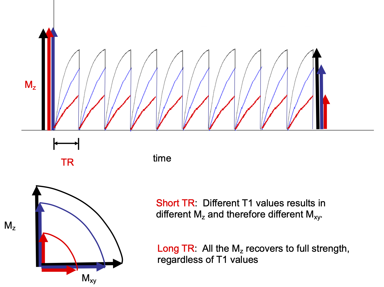
A 90 degrees RF pulse rotates all the longitudinal magnetization into the transverse plane resulting in zero longitudinal magnetization which then begins to recover. If TR is long compared to tissue T1 there is full recovery of longitudinal magnetization for each tissue before subsequent RF pulses. See Figure 2.

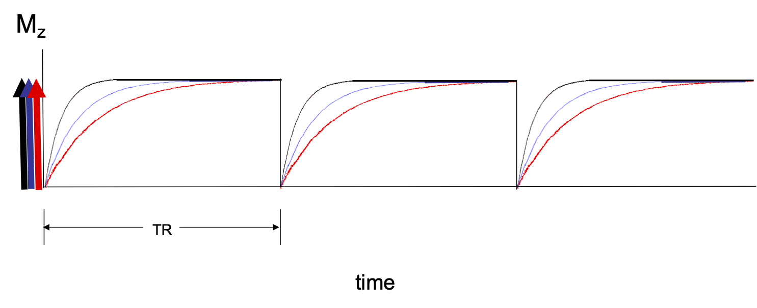
For TR on the order of tissue T1s the longitudinal magnetization of different tissues incomplelely recover prior the next RF pulse. After each RF pulse each tissue will have a different transverse magnetization or signal. See Figure 3.

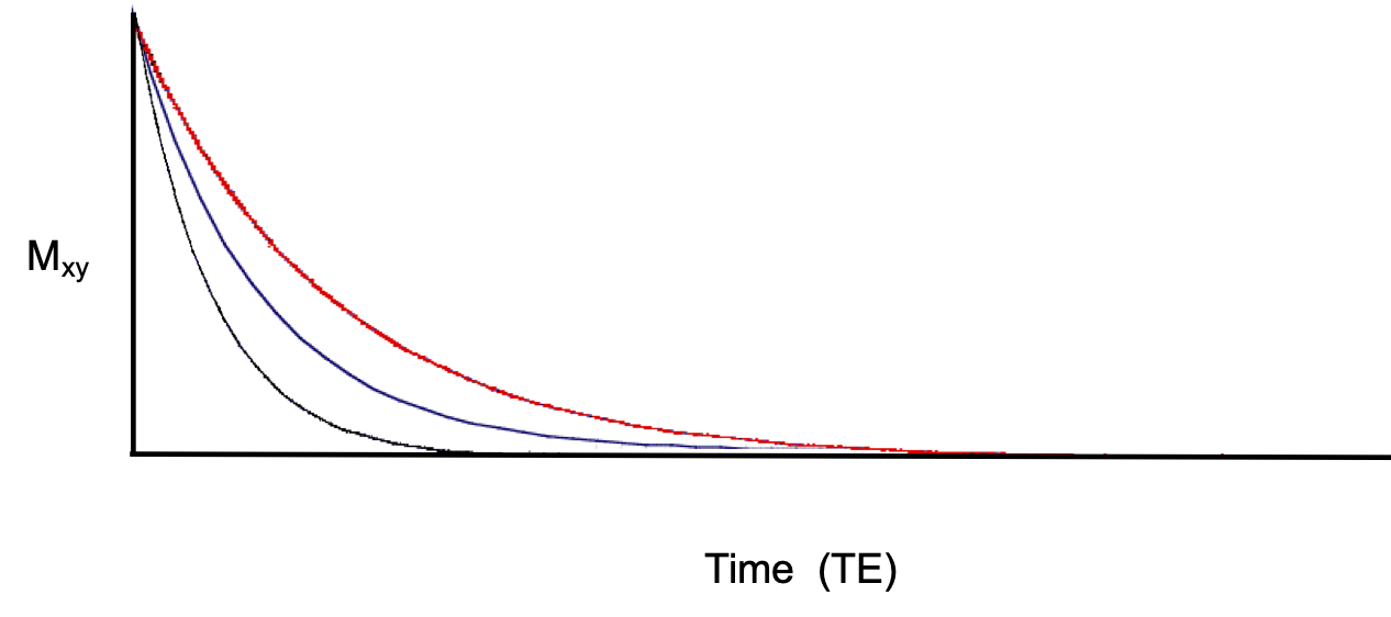
T2 relaxation is the process by which transverse magnetization, or signal, decays after an RF pulse. Transverse magetization decays based on the equation $M_{XY} = M_{XYo} e^{\frac{-t}{T2}}$ where t is time, T2 is the T2 is the T2 tissue property of the tissue, and $M_{XYo}$ is the the longitudinal magnetization of the tissue that was flipped into the transverse plane. See Figure 4.

Let's put this together.

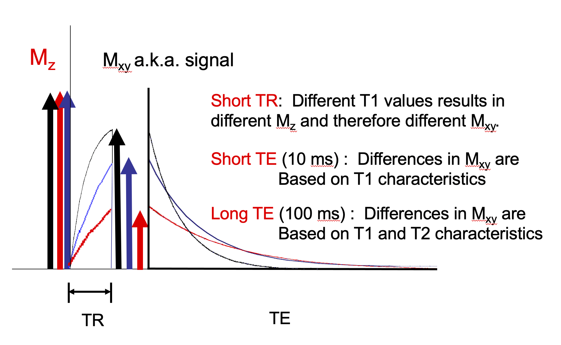
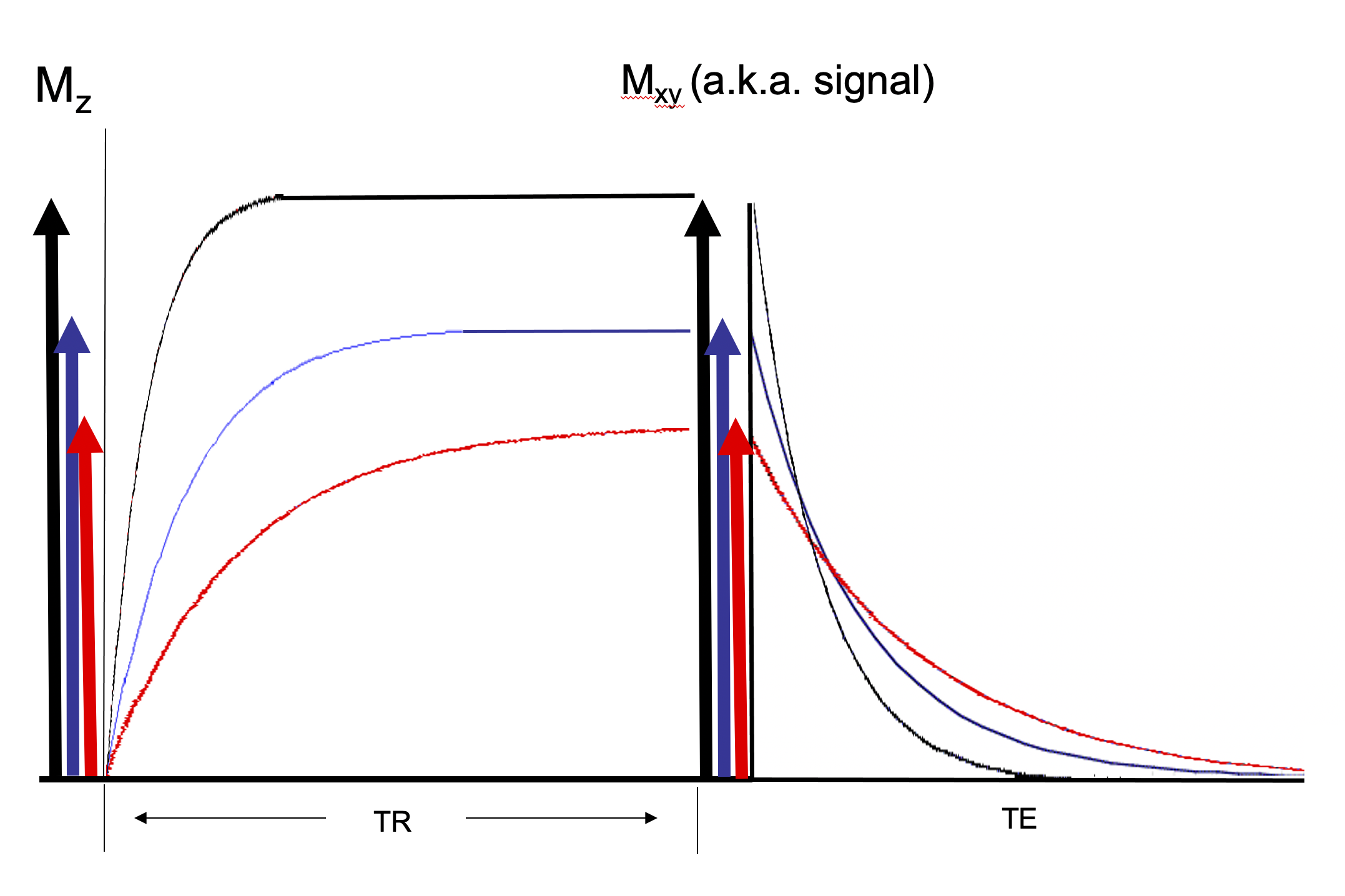
Choosing a short TR generates contrast between tissues based on their T1 values. Choosing a very short TE does not give the different tissues time to decay much which minimizes the contribution of T2 properties to the image. This is the basis of a "T1 weighted," image. See Figure 5.

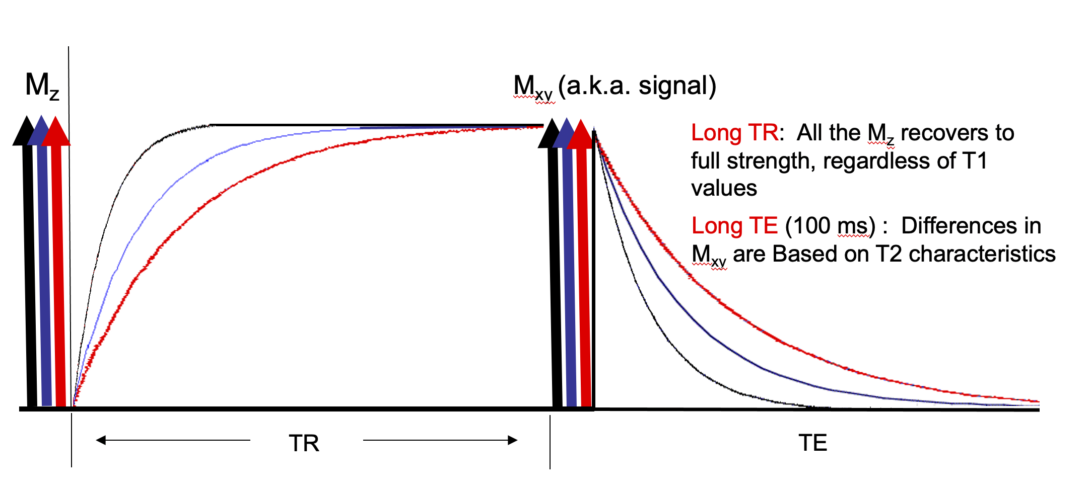
Choosing a long TR allows the longitudinal magnetization to fully recover which removes the contribution of T1 to signal. Choosing a mid range TE results in signal that is due to differences in T2. This is the basis of a "T2 weighed" image. See Figure 6.

The graphs just presented are not technically correct. We have ignored PD. Each tissue also has a different proton density which is the number of water protons per volume of tissue. The more protons per volume the more signal there is. The graph for the recovery of longitudinal magnetization should really look like Figure 7. Even at long TRs there are different longitudinal magnetizations for the different tissues due to their different proton density. A sequence with a long TR to remove contrast from the effects of different tissue T1s and with a short TE to remove contrast from the effects of different tissue T2s is a PD weighted sequence.

This is a great framework for conceptually explaining the basics of soft tissue contrast because it allows one to visualize what the spins in each tissue are doing for a given TR and TE. But it does not provide insight into optimising contrast between two tissues or, more importantly, optimising sensitivity to changes from normal in a specific tissue. To compare how tissues will look compared to each other one must create plots like the above figures for each tissue of interest AND create a separate figure for every possible combination of TR and TE. For example, one could not use this framework to answer the question: "What are the optimal parameters for looking for subtle changes in the T2 of normal white matter." This becomes even more complicated when introducing other tissue properties such as diffusion and susceptibility.

The following sections introduce a better framework for understanding the tissue contrast produced by an image called tissue property filters. This framework provides a basis for understanding more complex pulse sequences and for understanding the synergistic use of multiple tissue properties in the same sequence to increase contrast. Using this framework it is straightforward to visualize how changes in parameters affect tissue contrast. It will eventually become apparent that the current nomenclature of "T1" vs "T2" vs "PD" weighting is misleading, and that for a given TR and TE an image may be T1 weighted for one tissue but T2 weighted for another! We firmly believe that a better understanding of an image results in a better interpretation of the image.